In this post, I’ll review a paper from 2018 that deals with generating boolean decision rules and uses column generation. The paper is well worth the read if you are interested in explainable AI models. The work also won the FICO explainability challenge by applying this method to data from the financial services sector.

Setting

Algorithmic decisions - ones where you rely on machines to reach a conclusion - require justification. Why was my loan approval denied? Why was the scan result classified as cancerous? In these and several other critical sectors, simply stating the prediction of a AI system is not enough. The underlying rationale of “why” is equally important.

Several methods seek to come up with the justification algorithmically (in a field called Explainable AI) and several methods exist that can be distinguished along several dimensions. The main one is scope. The global methods look to explain the entire model, i.e. how does the model behave? This contrasts with local methods that look to explain a single instance, i.e. why was my loan not approved?

When the models are complex, as is often the case, a popular class of methods are surrogate models. The basic goal here is to build a simpler (e.g. linear) version of a complex model, then look to interpret the simpler model in ways we humans can understand. When built for local explanations, these probe the neighborhood of test instance to build a surrogate of the complex model.

Unfortunately, it is hard to be objective when it comes to explanations. In practice, different methods will result in vastly different explanations for the same instance on the same underlying (complex) model. For minor changes in training samples or an adjustment of parameters, even the same method can give you very different results. Fundamentally, these approaches are limited by design. If you prescribe to the view that a machine learning (ML) model is all but a lossy compressed view on the data, then surrogate models are a lossy compressed view of the ML model. Significant challenges remain in practical deployments.

An alternative view, the one described in the paper, is one where the model is directly interpretable. A directly interpretable model is one that can be understood by humans. There are of course, several models like decision trees that fall in this category.

The problem

Consider a supervised binary classification task. You are given $(X_i, y_i)$ for observations $i = 1,…, n$, where $X_i$ is the set of features associated with observation $i$ and $y_i$ is the binary outcome label. The task is to build a boolean classifier $\hat{y}(\mathbf{x})$ that can be stated as

if (condition) then (predict True) else (predict False)

where (condition) is of a specific form called a Disjunctive Normal Form (DNF). DNF clauses are OR of ANDs. A DNF clause on when to drink beer would be (mood=HAPPY AND inventory>0) OR (mood=SAD AND inventory>0) OR (temp>15°C).

For a dataset there are exponentially many such clauses involving its features. The challenge is to find a relatively compact subset that provides the best prediction accuracy. The condition needs to be compact as overly complex clauses are not interpretable.

The model

The paper formulates the search for these clauses as a mixed-integer programming problem.

$P$ denotes the set of positive samples, i.e. the observations where $y_i = 1$ and $Z$ denote negative ones. All features in $X_i$ are assumed to be binary valued. This isn’t too restrictive, continuous and categorical data can be encoded this way. There is $K$ a set of (exponentially many) clauses involving features of $X$ and $K_i, K_i\subseteq K$ is the subset of clauses satisfied by observation $i$.

There are two decision variables. First is $w_k$ (for all $k$ in set $K$) - a binary variable on if clause $k$ is selected for the model. Each clause $k$ in $K$ has an associated complexity $c_k$. The second is $\xi_i$ defined for $i \in P$ (i.e. for all positive samples) denotes all samples that are classified incorrectly.

The objective looks to minimize Hamming loss which is the fraction of misclassified samples. Specifically, this can be written as

$$ \min_{\xi, w} \color{blue}\underbrace{\color{black}\sum_{i\in P} \xi_i}{\text{false negatives}} {\color{black}+} \color{blue}\underbrace{\color{black}\sum{i\in Z}\sum_{k\in K_i} w_k}_{\text{false positives}} $$

False positives add more than “one unit” if multiple clauses are satisfied. This is

$$\begin{aligned} \mbox{s.t.} \qquad & \xi_i + \sum_{k\in K_i} w_k \ge 1 \qquad \xi_i \ge 0, \qquad i\in P \\ & \sum_{k\in K} c_k w_k \le C \\ & w_k \in \{0, 1\} \qquad \forall k\in K \end{aligned} $$

The first constraint looks to identify false negatives. It basically says, for each positive sample, either chalk up a false negative ($\xi_i$) or include a rule that correctly represents this observation (i.e. a clause from the set $K_i$). The second constraint simply bounds the total complexity of the selected rule set to a parameter $C$.

The overall problem still remains however, the set $K$ is very large and we’d like to avoid having to generate the entire set. This mainly because, it is expensive to generate and solve for all $K$. In any case, only a few $w_k$ will be selected in the final solution, so it makes sense to only look at clauses as needed.

In the maximum clique post earlier, this type of exponential growth was addressed using constraint generation. In this work, they follow a column generation procedure - one of generating new variables ($w_k$) as needed. Adding rows and columns to a optimization program are strongly coupled topics. Adding a constraint (row) to a program is the same as adding a variable (column) to its dual.

The pricing problem

Now to the problem of generating new conjunctive clauses. The sub-problem looks to find the missing clause with the highest reduced cost, i.e. the clause that has the greatest impact on the objective function. This is a heuristic selection and you may have to undo a selection at a later step. But if no missing clause with a negative reduced cost can be found, the procedure terminates with the optimal solution.

A bit more notation. From the program above, take $\mu_i$ to be the dual variables associated with the first constraint, and $\lambda$ be the dual variable for the complexity constraint. Define two sets of decision variables $\delta_i$ for all observations $i$ and $z_j$ if feature $j\in J$ is selected in missing constraint. Additionally denote $S_i$ to be a set of zero valued features for sample $i$.

Armed with this, the sub-problem to identify a clause to include (with the greatest negative reduce cost) can be formulated as:

$$ \min_{\delta, z} \color{blue}\underbrace{\color{black}\lambda\left(1+\sum_{j\in J}z_j\right)}{\substack{\text{complexity of new rule}\\\text{in terms of features selected}}} {\color{black}-} \color{blue}\underbrace{\color{black}\sum{i\in P} \mu_i \delta_i}{\substack{\text{how much the new rule}\\\text{improves false negatives}}}{\color{black}+} \color{blue}\underbrace{\color{black}\sum{i\in Z} \delta_i}_{\substack{\text{how much the new rule}\\\text{hurts false positives}}} $$

$$\begin{aligned} \mbox{s.t.} \qquad & \delta_i + z_j\le 1 \qquad j\in S_i, \qquad i\in P \\ & \delta_i \ge 1- \sum_{j\in S_i} z_j \qquad \delta_i\ge 0 \qquad i\in Z\\ & \sum_{j\in J} z_j \le D \\ & z_j \in \{0, 1\} \qquad \forall j\in J \end{aligned} $$

The first constraint here says every zero-valued feature in every positive sample - the feature is either selected or the sample satisfies the clause. The next constraint states that the $i$-th negative sample is covered only if no zero-valued feature is selected. The next constraint bounds the complexity and the feature selection variables are restricted to be binary.

Conclusions

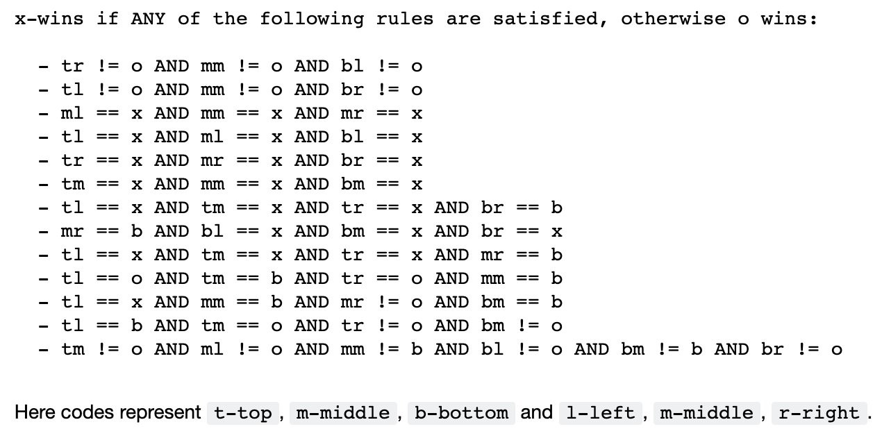
The method appears to be well suited for transactional-type data, where there are some underlying rules (e.g. a business process) that generates the training data. I leave you with an interesting example. The tic-tac-toe dataset contains all possible board configurations at the end of a tic-tac-toe game and the outcome (if x won or not). The method extracts almost all the rules of the game based on just this data, just missing the diagonal cases. Some of the rules extracted are superfluous.

As with all things, the approach comes with some limitations. There is a complexity-accuracy tradeoff, expect classifier accuracy to drop. Although in my experiments this was not substantial. The clauses generated are sensitive to the parameter $C$. If you don’t have a mechanism to validate the rule set then it is difficult to tune. The method doesn’t deal with class-imbalance, so you would need to under/over-sample to get a balanced sample. It would also worthwhile to study clauses generated in the presence of highly correlated features. I expect one of the correlated features to be picked arbitrarily.

Resources

A modified implementation of the model is available through the AIX360 toolkit, so you can try it yourself. The differences are documented in another paper. Mainly, it uses a beam search heuristic instead of the pricing problem. Additionally, the complexity clauses are handled through two regularization terms, rather than a constraint.